Quick start with SpharaPy

Section contents

In this tutorial, we briefly introduce the vocabulary used in spatial harmonic analysis (SPHARA) and we give a simple learning example to SpharaPy.

SPHARA – The problem setting

Fourier analysis is one of the standard tools in digital signal and image processing. In ordinary digital image data, the pixels are arranged in a Cartesian or rectangular grid. Performing the Fourier transform, the image data \(x[m,n]\) is compared (using a scalar product) with a two-dimensional Fourier basis \(f[k,l] = \mathrm{e}^{-2\pi \mathrm{i} \cdot \left(\frac{mk}{M} + \frac{nl}{N} \right) }\). In Fourier transform on a Cartesian grid, the Fourier basis used is usually inherently given in the transformation rule

\[X[k,l] = \sum_{m=0}^{M-1} \sum_{n=0}^{N-1} x[m,n] \cdot \mathrm{e}^{-2\pi \mathrm{i} \cdot \left(\frac{mk}{M} + \frac{nl}{N} \right) }\,.\]

A Fourier basis is a solution to Laplace’s eigenvalue problem (related to the Helmholtz equation)

\[L \vec{x} = \lambda \vec{x}\,,\qquad\qquad(1)\]

with the discrete Laplace-Beltrami operator in matrix notation \(L \in \mathbb{R}^{M \times N}\), the eigenvectors \(\vec{x}\) containing the harmonic functions and the eigenvalues \(\lambda\) the natural frequencies.

An arbitrary arrangement of sample points on a surface in three-dimensional space can be described by means of a triangular mesh. A spatial harmonic basis (SPHARA basis) is a solution of a Laplace eigenvalue problem for the given triangle mesh can be obtained by discretizing a Laplace-Beltrami operator for the mesh and solving the Laplace eigenvalue problem in equation (1). SpharaPy provides classes and functions to support these tasks:

• managing triangular meshes describing the spatial arrangement of the sample points,

• determining the Laplace-Beltrami operator of these meshes,

• computing a basis for spatial Fourier analysis of data defined on the triangular mesh, and

• performing the SPHARA transform and filtering.

The SpharaPy package

The SpharaPy package consists of five modules spharapy.trimesh, spharapy.spharabasis, spharapy.spharatransform, spharapy.spharafilter and spharapy.datasets. In the following we use three of the five SpharaPy modules to briefly show how a SPHARA basis can be calculated for given spatial sample points. The spharapy.trimesh module contains the TriMesh class, which can be used to specify the configuration of the spatial sample points. The SPHARA basis functions can be determined using the spharapy.spharabasis module, employing different discretizations. The spharapy.datasets module is an interface to the example data sets provided with the SpharaPy package.

# Code source: Uwe Graichen
# License: BSD 3 clause

# import modules from spharapy package
import spharapy.trimesh as tm
import spharapy.spharabasis as sb
import spharapy.datasets as sd

# import additional modules used in this tutorial
import matplotlib.pyplot as plt
from mpl_toolkits.mplot3d import Axes3D
import numpy as np

Specification of the spatial configuration of the sample points

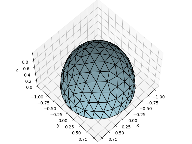
To illustrate some basic functionality of the SpharaPy package, we load a simple triangle mesh from the example data sets.

# loading the simple mesh from spharapy sample datasets
mesh_in = sd.load_simple_triangular_mesh()

The imported mesh is defined by a list of triangles and a list of vertices. The data are stored in a dictionary with the two keys ‘vertlist’ and ‘trilist’

print(mesh_in.keys())

Out:

dict_keys(['vertlist', 'trilist'])

The simple, triangulated surface consists of 131 vertices and 232 triangles and is the triangulation of a hemisphere of an unit ball.

vertlist = np.array(mesh_in['vertlist'])
trilist = np.array(mesh_in['trilist'])
print('vertices = ', vertlist.shape)
print('triangles = ', trilist.shape)

Out:

vertices =  (131, 3)
triangles =  (232, 3)

fig = plt.figure()
fig.subplots_adjust(left=0.02, right=0.98, top=0.98, bottom=0.02)
ax = fig.gca(projection='3d')
ax.set_xlabel('x')
ax.set_ylabel('y')
ax.set_zlabel('z')
ax.view_init(elev=60., azim=45.)
ax.set_aspect('auto')
ax.plot_trisurf(vertlist[:, 0], vertlist[:, 1], vertlist[:, 2],
                triangles=trilist, color='lightblue', edgecolor='black',
                linewidth=1)

Out:

/home/docs/checkouts/readthedocs.org/user_builds/spharapy/checkouts/latest/examples/plot_01_quick_start.py:123: MatplotlibDeprecationWarning: Calling gca() with keyword arguments was deprecated in Matplotlib 3.4. Starting two minor releases later, gca() will take no keyword arguments. The gca() function should only be used to get the current axes, or if no axes exist, create new axes with default keyword arguments. To create a new axes with non-default arguments, use plt.axes() or plt.subplot().
  ax = fig.gca(projection='3d')

<mpl_toolkits.mplot3d.art3d.Poly3DCollection object at 0x7f677070f950>

Determining the Laplace-Beltrami Operator

In a further step, an instance of the class spharapy.trimesh.TriMesh is created from the lists of vertices and triangles. The class spharapy.trimesh.TriMesh provides a number of methods to determine certain properties of the triangle mesh required to generate the SPHARA basis.

# print all implemented methods of the TriMesh class
print([func for func in dir(tm.TriMesh) if not func.startswith('__')])

Out:

['adjacent_tri', 'is_edge', 'laplacianmatrix', 'massmatrix', 'one_ring_neighborhood', 'remove_vertices', 'stiffnessmatrix', 'trilist', 'vertlist', 'weightmatrix']

# create an instance of the TriMesh class
simple_mesh = tm.TriMesh(trilist, vertlist)

For the simple triangle mesh an instance of the class SpharaBasis is created and the finite element discretization (‘fem’) is used. The complete set of SPHARA basis functions and the natural frequencies associated with the basis functions are determined.

sphara_basis = sb.SpharaBasis(simple_mesh, 'fem')
basis_functions, natural_frequencies = sphara_basis.basis()

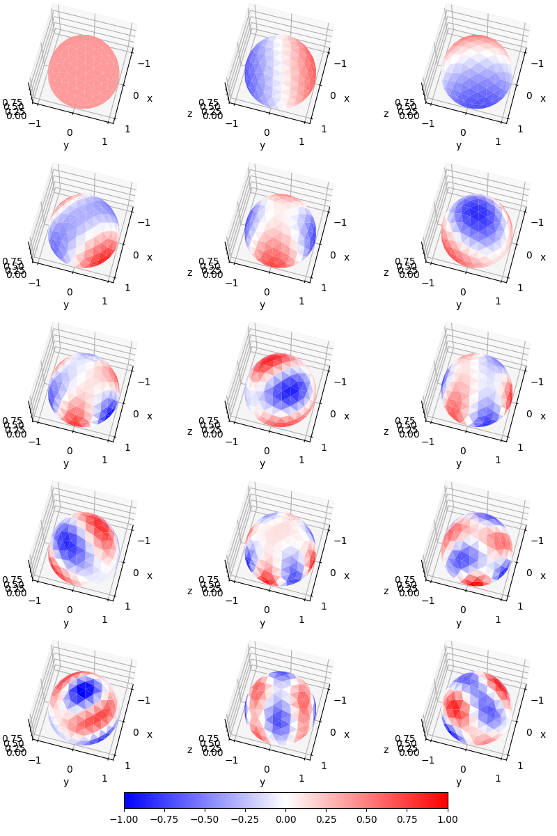
The set of SPHARA basis functions can be used for spatial Fourier analysis of the spatially irregularly sampled data.

The first 15 spatially low-frequency SPHARA basis functions are shown below, starting with DC at the top left.

# sphinx_gallery_thumbnail_number = 2
figsb1, axes1 = plt.subplots(nrows=5, ncols=3, figsize=(8, 12),
                             subplot_kw={'projection': '3d'})
for i in range(np.size(axes1)):
    colors = np.mean(basis_functions[trilist, i + 0], axis=1)
    ax = axes1.flat[i]
    ax.set_xlabel('x')
    ax.set_ylabel('y')
    ax.set_zlabel('z')
    ax.view_init(elev=70., azim=15.)
    ax.set_aspect('auto')
    trisurfplot = ax.plot_trisurf(vertlist[:, 0], vertlist[:, 1],
                                  vertlist[:, 2], triangles=trilist,
                                  cmap=plt.cm.bwr,
                                  edgecolor='white', linewidth=0.)
    trisurfplot.set_array(colors)
    trisurfplot.set_clim(-1, 1)

cbar = figsb1.colorbar(trisurfplot, ax=axes1.ravel().tolist(), shrink=0.75,
                       orientation='horizontal', fraction=0.05, pad=0.05,
                       anchor=(0.5, -4.0))

plt.subplots_adjust(left=0.0, right=1.0, bottom=0.08, top=1.0)
plt.show()