SPHARA – The theoretical background in a nutshell

Motivation

The discrete Fourier analysis of 2D data defined on a flat surface and represented by a Cartesian or a regular grid is very common in digital image processing and a fundamental tool in many applications. For such data, the basis functions (BF) for the Fourier transformation are usually implicitly specified in the transformation rule, compare [RKH10].

However, in many applications the sensors for data acquisition are not located on a flat surface and can not be represented by Cartesian or regular grids. An example from the field of biomedical engineering for non-regular sensor positions is the electroencephalography (EEG). In EEG, the sensors are placed at predetermined positions at the head surface, a surface in space \(\mathbb{R}^3\). The positions of the sensors of these systems can be described by means of triangular meshes. Because of the particular sensor arrangement, the spatial analysis of multi-sensor data can not be performed using the standard 2D Fourier analysis. However, a spatial Fourier analysis can be also very useful for spatially irregularly sampled data.

In this Python package we implement a new method for SPatial HARmonic Analysis (SPHARA) of multisensor data using the eigenbasis of the Laplace-Beltrami operator of the meshed surface of sensor positions. Using this approach, basis functions of spatial harmonics for arbitrary arrangements of sensors can be generated. The recorded multisensor data are decomposed by projection into the space of the basis functions. For a much more detailed introduction of the theoretical principles of SPHARA see also [GEF+15].

Discrete representation of surfaces

For the discrete case we assume that the sensors are located on an arbitrary surface, which is represented by a triangular mesh in \(\mathbb{R}^3\). The mesh \(M = \{V,E,T\}\) consists of vertices \(v \in V\), edges \(e \in E\) and triangles \(t \in T\). Each vertex \(v_i \in \mathbb{R}^3\) represents a sensor position. The number of vertices, edges and triangles of \(M\) are defined by \(|V|\), \(|E|\) and \(|T|\), respectively. The neighborhood \(i^{\star}\) for a vertex \(v_i \in V\) is defined by \(i^{\star} = \{v_x \in V: e_{ix} \in E\}\), see Fig. 1 (b). The number of neighbors of \(v_i\) is \(n_i = |i^{\star}|\). The angles \(\alpha_{ij}\) and \(\beta_{ij}\) are located opposed to the edge \(e_{ij}\). The triangles \(t_a\) and \(t_b\), defined by the vertices \((v_i, v_j, v_o)\) and \((v_i, v_k, v_j)\), share the edge \(e_{ij}\). The set of triangles sharing the vertex \(v_i\) is given by \(i^{\triangledown} = \{t_x \in T : v_i \in t_x\}\). The area of a triangle \(t\) is given by \(|t|\). An example for these mesh components is illustrated in Fig. 1 (b).

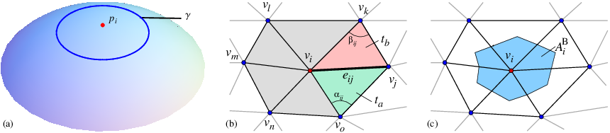
Fig. 1 The approximation of the Laplace-Beltrami operator. (a) continuous representation; (b) discrete representation. The neighborhood \(i^{\star}\) of vertex \(v_i\) consists of the vertices \(\{v_x \in V: e_{ix} \in E\}\). Either the length of \(e_{ij}\) or the size of the two angles \(\alpha_{ij}\) and \(\beta_{ij}\) opposed to the edge \(e_{ij}\) are used to estimate the weight \(w(i,j)\) for \(e_{ij}\). The two triangles \(t_a\) and \(t_b\) both share the edge \(e_{ij}\); (c) the area of the barycell \(A^{\mathrm{B}}_i\) for the vertex \(v_i\).

Discrete Laplace-Beltrami Operators

A function \(\vec{f}\) is defined for all vertices \(v_i \in V\), it applies \(\vec{f}: v_i \rightarrow \mathbb{R}\) with \(i = 1, \ldots, |V|\). A discretization \(\Delta_D\) of the Laplace-Beltrami operator for \(\vec{f}\) is given by

(1)\[\Delta_D \vec{f}_i = b^{-1}_i\sum_{x \in i^{\star}} w(i, x)\left(\vec{f}_i - \vec{f}_x\right)\,,\]

with the weighting function \(w(i, x)\) for edges \(e_{ix} \in E\) and the normalization coefficient \(b_i\) for the vertex \(v_i\). For practical applications it is convenient to transform equation (1) into matrix notation. The elements of the matrices \(B^{-1}\) and \(S\) are determined using the coefficients \(b_i\) and \(w(i, x)\) of equation (1). \(B^{-1}\) is a diagonal matrix, the elements are

(2)\[\begin{split}B^{-1}_{ij} = \begin{cases} b^{-1}_i & \text{if}\quad i = j\\ 0 & \text{otherwise}\,, \end{cases}\end{split}\]

and the entries of \(S\) are

(3)\[\begin{split}S_{ij} = \begin{cases} \sum_{x \in i^{\star}} w(i, x) & \text{if}\quad i = j\\ -w(i, x) & \text{if}\quad e_{ix} \in E\\ 0 & \text{otherwise}\,. \end{cases}\end{split}\]

A Laplacian matrix \(L\) can be expressed as product of a diagonal matrix \(B^{-1}\) and a matrix \(S\)

(4)\[L = B^{-1} \, S\,,\]

compare also [ZvKD10]. The size of the Laplacian matrix \(L\) for a mesh \(M\) is \(n \times n\), with \(n=|V|\). Using the Laplacian matrix L, \(\Delta_D\) applied to \(\vec{f}\) can be written as

(5)\[\Delta_D \vec{f} = - L \vec{f}\,.\]

In the following we present four different approaches to discretize the Laplace-Beltrami operator, a graph-theoretical approach and three geometric approaches.

First, we look at the graph-theoretical approach, where the coordinates of the positions of the vertices are not considered. The topological Laplacian results from equation (1) by using \(w(i,x) = b^{-1}_i = 1\), see also [Tau95][Chu97][ZvKD07]. The graph-theoretical approach will be referred to as TL later in the text.

Second, for inhomogeneous triangular meshes, where the distances between vertices and the sizes of angles and triangles are different, the weighting function \(w\) has to be adapted according to the mesh geometry. In these approaches, the positions of the vertices are also considered. They are referred to as geometric approaches. There are different approaches to treat inhomogeneous meshes.

The first possibility is to use the Euclidean distance of adjacent vertices raised to the power of a value \(\alpha\). For equation (1) the coefficients \(b^{-1}_i = 1\) and \(w(i, x) = ||e_{ix}||^{\alpha}\) are chosen. A common choice is to use the inverse of the Euclidean distance with \(\alpha = -1\) [Tau95][Fuj95]. This approach will be referred to later as IE.

The second approach for a geometric discretization of the Laplace-Beltrami operator is derived by minimizing the Dirichlet energy for a triangulated mesh [PP93][Pol02]. It uses cotangent weights with

(6)\[w(i,x) = \frac{1}{2}\left(\cot(\alpha_{ix}) + \cot(\beta_{ix})\right)\,,\]

with the two angles \(\alpha_{ix}\) and \(\beta_{ix}\) opposed to the edge \(e_{ix}\), see Fig. 1 (b). For edges on the boundary of the mesh, the term \(\cot(\beta_{ix})\) is omitted, which leads to Neumann Boundary condition (BC). A drawback of using the cotangent weights is that the value representing the integral of the Laplacian over a 1-ring neighborhood (area of the \(i^{\star}\)-neighborhood) is assigned to a point sample [ZvKD07]. To resolve this issue and to guarantee the correspondence between the continuous and the discrete approaches, the weights in equation (6) are divided by the area \(A^{\mathrm{B}}_i\) of the barycell for the vertex \(v_i\) [MDSB03], resulting in

(7)\[w(i,x) = \frac{1}{2 A^{\mathrm{B}}_i}\left(\cot(\alpha_{ix}) + \cot(\beta_{ix})\right)\,.\]

The barycell for a vertex \(v_i\) is framed by a polygonal line that connects the geometric centroids of triangles in \(i^{\triangledown}\) and the midpoints of the adjoined edges \(e_{ix}\), see Fig. 1 (c). The area of the \(i^{\star}\)-neighborhood for a vertex \(v_i\), which is the area of the triangles that are enclosed by the vertices \(v_x \in i^{\star}\), is referred to as \(A^1_i\). Then \(A^{\mathrm{B}}_i\) can be determined by \(A^{\mathrm{B}}_{i} = \frac{1}{3} A^1_i\). For the discretizations using the cotangent weighted formulation, the parameter \(b^{-1}_i\) in equation (1) is set to \(b^{-1}_i = 1\). This approach, using cotangent weights will be referred to as COT later in the manuscript.

The third geometric approach to discretize the Laplace-Beltrami operator is the Finite Element Method (FEM), which is related to the approach using cotangent weights. Assuming that the function \(f\) is piecewise linear and defined by its values \(f_i\) on the vertices \(v_i\) of a triangular mesh, \(f\) can be interpolated using nodal basis functions \(\psi_i\)

(8)\[f = \sum_{i = 1}^{|V|} f_i \, \psi_i\,.\]

We use the hat function for \(\psi_i\), with

(9)\[\begin{split}\psi_i(j) = \begin{cases} 1 & \text{if}\quad i = j\\ 0 & \text{otherwise}\,. \end{cases}\end{split}\]

For two functions \(f\) and \(g\) defined on \(M\), a scalar product is given by

(10)\[\int_{M} f g \; \mathrm{d} a = \sum_{i = 0}^{|V|} \sum_{j = 0}^{|V|} f_i g_i \int_{M} \psi_i \psi_j \;\mathrm{d} a = \left\langle \vec{f}, \vec{g} \right\rangle_B\,,\]

with the area element \(\mathrm{d} a\) on \(M\) and the mass matrix \(B\). The sparse mass matrix \(B\) is given by

(11)\[B_{ij} = \int_{M} \psi_i \psi_j \,\mathrm{d} a\,.\]

For the FEM approach using hat functions, the elements of \(B\) can be calculated by

(12)\[\begin{split}B_{ij} = \begin{cases} \left( \sum_{t \in i^{\triangledown}} |t|\right) / 6 & \text{if}\quad i = j\\ \left(|t_a| + |t_b| \right) / 12 & \text{if}\quad e_{ij} \in E\\ 0 & \text{otherwise}\,, \end{cases}\end{split}\]

where \(t_a\) and \(t_b\) are the two triangles adjacent to the edge \(e_{ij}\), see Fig. 1 (b). For the FEM discretization of the Laplace-Beltrami operator also a stiffness matrix \(S\) has to be calculated. The elements of \(S_{ij}\) can be estimated using the equations (3) and (6), compare [DZMC07][ZvKD07][VL07].

Eigensystems of Discrete Laplace-Beltrami Operators

Desirable properties of the discrete Laplacian \(L\) are symmetry, positive weights, positive semi-definiteness, locality, linear precision and convergence [WMKG07]. The symmetry \(L_{ij} = L_{ji}\) leads to real eigenvalues and orthogonal eigenvectors. Positive weights \(w(i,j) \ge 0\) assure, together with the symmetry, the positive semi-definiteness of \(L\). The locality of the discrete Laplace-Beltrami operator enables the determination of weights \(w(i,j)\) using the \(i^{\star}\)-neighborhood of a vertex \(v_i\), with \(w(i,j) = 0\), if \(e_{ij} \notin E\). The linear precision implies for a linear function \(f\) defined on vertices \(v_i\) that \(\Delta_{D} \vec{f}_i = 0\) applies, which ensures the exact recovery of \(f\) from the samples. The convergence property provides the convergence from the discrete to the continuous Laplace-Beltrami operator \(\Delta_D \rightarrow \Delta\) for a sufficient refinement of the mesh.

The Laplacian matrix \(L\) for the TL and the IE approach are positive semi-definite, symmetric and use positive weights. The COT and the FEM approach do not fulfill the positive weight property, if the mesh contains triangles with interior angles in the interval \((\pi/2, \pi)\), for which the cotangent is negative. The TL approach is no geometric discretization, because it violates the linear precision and the convergence property. In contrast, the COT and the FEM approach are geometric discretizations as they fulfill the linear precision and the convergence property, but they violate the symmetry property. None of the presented discretization methods fulfill all desirable properties, see also [WMKG07].

The discrete Laplacian eigenvalue problem for a real and symmetric Laplacian matrix is given by

(13)\[L \, \vec{x}_i = \lambda_i \, \vec{x}_i\,,\]

with eigenvectors \(\vec{x}_i\) and eigenvalues \(\lambda_i\) of \(L\). The Laplacian matrix \(L\) is real and symmetric for the TL, the IE and the COT approach. Because \(L\) is real and symmetric, eigenvalues \(\lambda_i \in \mathbb{R}\) with \(\lambda_i \ge 0\) are obtained. The eigenvectors \(\vec{x}_i\) are real-valued and form a harmonic orthonormal basis. The corresponding eigenvalues \(\lambda_i\) can be considered as spatial frequencies. The eigenvectors \(\vec{x}_i\) can be used for a spectral analysis of functions defined on the mesh \(M\). The projection of a discrete function \(\vec{f}\) defined on \(M\) onto the basis of spatial harmonic functions is performed by the inner product for Euclidean \(n\)-spaces \(\langle\vec{f}, \vec{x}_i\rangle\). For the matrix \(X\), where the eigenvectors \(\vec{x}_i\) represent the columns,

\[X = [\vec{x}_1 \; \vec{x}_2 \cdots \vec{x}_n]\,,\]

it applies

(14)\[X^\top X = I\,,\]

with the identity matrix \(I\).

For the FEM formulation, the BF \(\vec{y}_i\) are computed by solving the generalized symmetric definite eigenproblem

(15)\[S \vec{y}_i = \lambda_i B \vec{y}_i\,.\]

Thus, the inversion of the mass matrix \(B\) is avoided. Because \(B^{-1}S\) is not symmetric, the eigenvectors \(\vec{y}_i\) are real-valued, but not orthonormal with respect to the inner product for Euclidean \(n\)-spaces \(\left\langle . \right\rangle\). To use these eigenvectors as BF, the inner product, defined in equation~(ref{eq:scalarproductfem}), has to be used

(16)\[\left\langle \vec{f}, \vec{y}_i \right\rangle_B = \vec{f}^{\,\top} B \, \vec{y}_i\,,\]

which assures the \(B\)-orthogonality, compare also cite{vallet07}. The eigenvectors computed by the FEM approach can be normalized by using the \(B\)-relative norm

(17)\[\vec{\tilde{y}}_i = \frac{\vec{y}_i}{\lVert\vec{y}_i\rVert_{B}} \quad \text{with} \quad \lVert\vec{y}_i\rVert_{B} = \sqrt{\left\langle \vec{y}_i, \vec{y}_i \right\rangle_B}\,.\]

For a matrix \(\tilde{Y}\), where the normalized eigenvectors \(\vec{\tilde{y}}_i\) represent the columns

(18)\[\tilde{Y} = [\vec{\tilde{y}}_1 \; \vec{\tilde{y}}_2 \cdots \vec{\tilde{y}}_n]\,,\]

it applies

(19)\[\tilde{Y}^\top B \tilde{Y} = I\,.\]

SPHARA as signal processing framework

Requirements

To use the eigenvectors of the discrete Laplacian Beltrami operator in the context of a signal processing framework, it is necessary that they exhibit certain properties. The eigenvectors have to form a set of BF. An inner product for the decomposition and for the reconstruction of the data has to be defined, which is used for the transformation into the domain of the spatial frequencies and for the back-transformation into the spatial domain. To be utilized for practical applications, the transformation from the spatial domain into the spatial frequency domain has to have linear properties and should fulfill Parseval’s theorem.

Basis functions

A complete set of linearly independent vectors can be used as basis. For real and symmetric Laplacian matrices \(L\) the orthonormality of the eigenvectors is given inherently, see equations (13) and (14). For the FEM approach, the orthonormality of the eigenvectors is assured explicitly, see equations (15) to (19). The property of orthogonality includes the linear independence. To use the eigenvectors as BF, they must further fulfill the property of completeness. The completeness can be shown by the dimension theorem for vector spaces. The dimensionality is equal for both the spatial representation and the representation in the spatial frequency domain. For a mesh with \(n\) vertices, \(n\) unit impulse functions are used as BF for the spatial representation. For the same mesh, we obtain \(n\) discrete spatial harmonic functions (eigenvectors) for the representation using spatial frequencies. The calculated eigenvectors are orthonormal and complete; therefore, they can be used as orthonormal BF.

Analysis and synthesis

For the analysis of discrete data defined on the vertices of the triangular mesh, the inner product is used (transformation from spatial domain to spatial frequency domain). For an analysis using the eigenvectors of a symmetric Laplacian matrix \(L\) (TL, IE and COT), the vector space inner product is applied. The coefficient \(c_i\) for a single spatial harmonic BF \(\vec{x}_i\) can be determined by

(20)\[c_i = \langle\vec{f}, \vec{x}_i\rangle\,.\]

The transformation from the spatial into the spatial frequency domain is computed by

(21)\[\vec{c}^{\,\top} = \vec{f}^{\,\top} \, X\,.\]

For an analysis using eigenvectors computed by the FEM approach, the inner product that assures the \(B\)-orthogonality needs to be applied

(22)\[c_i = \left\langle \vec{f}, \vec{\tilde{y}}_i \right\rangle_B = \vec{f}^{\,\top} B \, \vec{\tilde{y}}_i\,.\]

The transformation from the spatial into the spatial frequency domain is then be computed by

(23)\[\vec{c}^{\,\top} = \vec{f}^{\,\top} B \, \tilde{Y}\,.\]

Discrete data are synthesized using the linear combination of the coefficients \(c_i\) and the corresponding BF \(\vec{x}_i\) or \(\vec{\tilde{y}}_i\)

(24)\[\vec{f} = \sum_{i = 1}^n c_i \, \vec{x}_i\]

or

(25)\[\vec{f}^{\,\top} = \vec{c}^{\,\top} \, \tilde{Y}^{\,\top}\,.\]

Spatial filtering using SPHARA

At the end of this short introduction we show the design of a spatial filter as a practical application of SPHARA. The prerequisite for the successful use of SPHARA-based filters is the separability of useful signal and interference in the spatial SPHARA spectrum. This applies, for example, to EEG. In EEG, the low-frequency SPHARA basis functions provide the main contribution to signal power. In contrast, single channel dropouts and spatially uncorrelated sensor noise exhibit an almost equally distributed spatial SPHARA spectrum, compare [GEF+15] and tutorial Spatial SPHARA analysis of EEG data.

A filter matrix \(F\) can be determined by

\[F = X \cdot R \cdot (X \cdot R)^{\intercal}\,.\]

The matrix \(X\) contains columnwise the SPHARA basis functions and the matrix \(R\) is a selection matrix, that contains an 1 on the main diagonal if the corresponding SPHARA basis function from \(X\) is chosen. All other elements of this matrix are 0.

If the Laplace-Beltrami Operator with FEM discretization is used to calculate the SPHARA basis functions, the mass matrix \(B\) must be added to the equation to compute the filter matrix

\[F_{\mathrm{FEM}} = B \cdot X \cdot R \cdot (X \cdot R)^{\intercal}\,.\]

The spatial SPHARA filter is applied to the data by multiplying the matrix containing the data \(D\) by the filter matrix \(F\)

\[\tilde{D} = D \cdot F\,.\]

The matrix \(D\) contains data, time samples in rows and spatial samples in columns and the matrix \(\tilde{D}\) the filtered data, see also tutorial Spatial SPHARA filtering of EEG data.