Spatial SPHARA analysis of EEG data

Section contents

This tutorial shows exemplarily the spatial SPHARA analysis of 256-channel EEG data. The FEM discretization of the Laplace-Beltrami operator is employed to calculate the SPHARA basic functions that are used for the SPHARA decomposition.

Introduction

As explained in SPHARA – The theoretical background in a nutshell and in the tutorial Determination of the SPHARA basis functions for an EEG sensor setup a spatial Fourier basis for a arbitrary sensor setup can be determined as solution of the Laplace’s eigenvalue problem dicretized for the considered sensor setup

\[L \vec{x} = \lambda \vec{x}\,,\]

with the discrete Laplace-Beltrami operator in matrix notation \(L \in \mathbb{R}^{M \times N}\), the eigenvectors \(\vec{x}\) containing the harmonic functions and the eigenvalues \(\lambda\) the natural frequencies.

The spatial Fourier basis determined in this way can be used for the spatial Fourier analysis of data recorded with the considered sensor setup.

For the anaylsis of discrete data defined on the vertices of the triangular mesh - the SPHARA transform - the inner product is used (transformation from spatial domain to spatial frequency domain). For an analysis using eigenvectors computed by the FEM approach, the inner product that assures the \(B\)-orthogonality needs to be applied.

For the reverse transformation, the discrete data are synthesized using the linear combination of the SPHARA coefficients and the corresponding SPHARA basis functions. More detailed information can be found in the section Analysis and synthesis and in [GEF+15].

At the beginning we import three modules of the SpharaPy package as well as several other packages and single functions of packages.

# Code source: Uwe Graichen
# License: BSD 3 clause

# import modules from spharapy package
import spharapy.trimesh as tm
import spharapy.spharatransform as st
import spharapy.datasets as sd

# import additional modules used in this tutorial
import matplotlib.pyplot as plt
from mpl_toolkits.mplot3d import Axes3D
import numpy as np

Import the spatial configuration of the EEG sensors and the SEP data

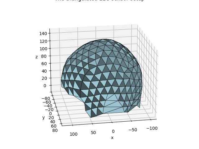
In this tutorial we will apply the SPHARA analysis to SEP data of a single subject recorded with a 256 channel EEG system with equidistant layout. The data set is one of the example data sets contained in the SpharaPy toolbox.

# loading the 256 channel EEG dataset from spharapy sample datasets
mesh_in = sd.load_eeg_256_channel_study()

The dataset includes lists of vertices, triangles, and sensor labels, as well as EEG data from previously performed experiment addressing the cortical activation related to somatosensory-evoked potentials (SEP).

print(mesh_in.keys())

Out:

dict_keys(['vertlist', 'trilist', 'labellist', 'eegdata'])

The triangulation of the EEG sensor setup consists of 256 vertices and 480 triangles. The EEG data consists of 256 channels and 369 time samples, 50 ms before to 130 ms after stimulation. The sampling frequency is 2048 Hz.

vertlist = np.array(mesh_in['vertlist'])
trilist = np.array(mesh_in['trilist'])
eegdata = np.array(mesh_in['eegdata'])
print('vertices = ', vertlist.shape)
print('triangles = ', trilist.shape)
print('eegdata = ', eegdata.shape)

Out:

vertices =  (256, 3)
triangles =  (482, 3)
eegdata =  (256, 369)

fig = plt.figure()
fig.subplots_adjust(left=0.02, right=0.98, top=0.98, bottom=0.02)
ax = fig.gca(projection='3d')
ax.set_xlabel('x')
ax.set_ylabel('y')
ax.set_zlabel('z')
ax.set_title('The triangulated EEG sensor setup')
ax.view_init(elev=20., azim=80.)
ax.set_aspect('auto')
ax.plot_trisurf(vertlist[:, 0], vertlist[:, 1], vertlist[:, 2],
                triangles=trilist, color='lightblue', edgecolor='black',
                linewidth=0.5, shade=True)
plt.show()

Out:

/home/docs/checkouts/readthedocs.org/user_builds/spharapy/checkouts/latest/examples/plot_03_sphara_analysis_eeg.py:105: MatplotlibDeprecationWarning: Calling gca() with keyword arguments was deprecated in Matplotlib 3.4. Starting two minor releases later, gca() will take no keyword arguments. The gca() function should only be used to get the current axes, or if no axes exist, create new axes with default keyword arguments. To create a new axes with non-default arguments, use plt.axes() or plt.subplot().
  ax = fig.gca(projection='3d')

x = np.arange(-50, 130, 1/2.048)
figeeg = plt.figure()
axeeg = figeeg.gca()
axeeg.plot(x, eegdata[:, :].transpose())
axeeg.set_xlabel('t/ms')
axeeg.set_ylabel('V/µV')
axeeg.set_title('SEP data')
axeeg.set_ylim(-3.5, 3.5)
axeeg.set_xlim(-50, 130)
axeeg.grid(True)
plt.show()

Create a SpharaPy TriMesh instance

In the next step we create an instance of the class spharapy.trimesh.TriMesh from the list of vertices and triangles.

# create an instance of the TriMesh class
mesh_eeg = tm.TriMesh(trilist, vertlist)

SPHARA transform using FEM discretisation

Create a SpharaPy SpharaTransform instance

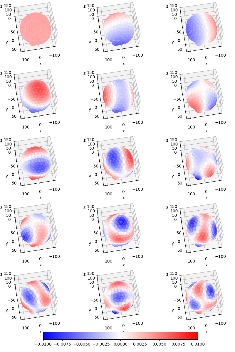
In the next step of the tutorial we determine an instance of the class SpharaTransform, which is used to execute the transformation. For the determination of the SPHARA basis we use a Laplace-Beltrami operator, which is discretized by the FEM approach.

sphara_transform_fem = st.SpharaTransform(mesh_eeg, 'fem')
basis_functions_fem, natural_frequencies_fem = sphara_transform_fem.basis()

Visualization the basis functions

The first 15 spatially low-frequency SPHARA basis functions of the basis used for the transform are shown below, starting with DC at the top left.

figsb1, axes1 = plt.subplots(nrows=5, ncols=3, figsize=(8, 12),
                             subplot_kw={'projection': '3d'})
for i in range(np.size(axes1)):
    colors = np.mean(basis_functions_fem[trilist, i + 0], axis=1)
    ax = axes1.flat[i]
    ax.set_xlabel('x')
    ax.set_ylabel('y')
    ax.set_zlabel('z')
    ax.view_init(elev=60., azim=80.)
    ax.set_aspect('auto')
    trisurfplot = ax.plot_trisurf(vertlist[:, 0], vertlist[:, 1],
                                  vertlist[:, 2], triangles=trilist,
                                  cmap=plt.cm.bwr,
                                  edgecolor='white', linewidth=0.)
    trisurfplot.set_array(colors)
    trisurfplot.autoscale()
    trisurfplot.set_clim(-0.01, 0.01)

cbar = figsb1.colorbar(trisurfplot, ax=axes1.ravel().tolist(), shrink=0.85,
                       orientation='horizontal', fraction=0.05, pad=0.05,
                       anchor=(0.5, -4.5))

plt.subplots_adjust(left=0.0, right=1.0, bottom=0.08, top=1.0)
plt.show()

SPHARA transform of the EEG data

In the final step we perform the SPHARA transformation of the EEG data. As a result, a butterfly plot of all channels of the EEG is compared to the visualization of the power contributions of the first 40 SPHARA basis functions. Only the first 40 out of 256 basis functions are used for the visualization, since the power contribution of the higher basis functions is very low.

# perform the SPHARA transform
sphara_trans_eegdata = sphara_transform_fem.analysis(eegdata.transpose())

# 40 low-frequency basis functions are displayed
ysel = 40
figsteeg, (axsteeg1, axsteeg2) = plt.subplots(nrows=2)

y = np.arange(0, ysel)
x = np.arange(-50, 130, 1/2.048)

axsteeg1.plot(x, eegdata[:, :].transpose())
axsteeg1.set_ylabel('V/µV')
axsteeg1.set_title('EEG data, 256 channels')
axsteeg1.set_ylim(-2.5, 2.5)
axsteeg1.set_xlim(-50, 130)
axsteeg1.grid(True)

pcm = axsteeg2.pcolormesh(x, y,
                          np.square(np.abs(sphara_trans_eegdata.transpose()
                                           [0:ysel, :])))
axsteeg2.set_xlabel('t/ms')
axsteeg2.set_ylabel('# BF')
axsteeg2.set_title('Power contribution of SPHARA basis functions')
axsteeg2.grid(True)
figsteeg.colorbar(pcm, ax=[axsteeg1, axsteeg2], shrink=0.45,
                  anchor=(0.85, 0.0), label='power / a.u.')

plt.subplots_adjust(left=0.1, right=0.85, bottom=0.1, top=0.95, hspace=0.35)
plt.show()
# sphinx_gallery_thumbnail_number = 4