SPHARA basis and transform on EEG data (BaCI 2019)

Based on the course materials from Training Course 4, held at the International Conference on Basic and Clinical Multimodal Imaging (BaCI) in Chengdu, China, in September 2019.

This tutorial introduces the basic steps of a SPHARA-based analysis using the SpharaPy toolbox:

• loading a triangulated EEG sensor layout,

• computing a SPHARA basis from a discrete Laplace–Beltrami operator,

• interpreting the eigenvalues as spatial wave numbers,

• deriving spatial frequencies and wavelengths, and

• computing the SPHARA transform of multichannel EEG data.

The example uses a 256-channel somatosensory evoked potential (SEP) data set. All steps are implemented with the high-level classes from spharapy:

• spharapy.trimesh.TriMesh

• spharapy.spharabasis.SpharaBasis

• spharapy.spharatransform.SpharaTransform

The corresponding theoretical background is described in more detail in the SPHARA introduction section of the documentation.

The example data set contains somatosensory-evoked potentials (SEP) measured with 256 EEG channels. The vertex positions of the EEG mesh are given in millimetres (mm), and the EEG amplitudes are measured in microvolts (µV). The recording contains 369 time samples from 50 ms before to 130 ms after stimulation at a sampling frequency of 2048 Hz.

Imports and dataset

We start by importing NumPy, Matplotlib, and the relevant SpharaPy modules. The example uses a convenience loader from spharapy.datasets which provides

• a triangulated EEG sensor mesh,

• SEP data of shape (n_channels, n_times), and

• channel labels.

import numpy as np
import matplotlib.pyplot as plt
from mpl_toolkits.mplot3d import Axes3D  # noqa: F401  (required for 3D plotting)

import spharapy.datasets as sd
import spharapy.trimesh as tm
import spharapy.spharabasis as sb
import spharapy.spharatransform as st

# Load example SEP data and EEG mesh
# ----------------------------------
#
# We use the same 256-channel SEP data set as in
# :mod:`examples.plot_04_sphara_filter_eeg`.  The loader returns a
# dictionary with vertex list, triangle list, EEG data and channel
# labels.

mesh_in = sd.load_eeg_256_channel_study()

print(mesh_in.keys())

# The triangulation of the EEG sensor setup consists of 256 vertices
# and 480 triangles. The EEG data consists of 256 channels and 369
# time samples, 50 ms before to 130 ms after stimulation. The sampling
# frequency is 2048 Hz.

vertlist = np.array(mesh_in["vertlist"])
trilist = np.array(mesh_in["trilist"])
labelist = np.array(mesh_in["labellist"])
eegdata = np.array(mesh_in["eegdata"])

# channel labels
channel_labels = labelist

print("vertices = ", vertlist.shape)
print("triangles = ", trilist.shape)
print("eegdata = ", eegdata.shape)

# build TriMesh and standardised variable names used later in the tutorial
mesh_eeg = tm.TriMesh(trilist, vertlist)
eeg_data = eegdata

n_channels, n_times = eeg_data.shape
print(f"Number of channels: {n_channels}")
print(f"Number of time samples: {n_times}")

dict_keys(['vertlist', 'trilist', 'labellist', 'eegdata'])
vertices =  (256, 3)
triangles =  (482, 3)
eegdata =  (256, 369)
Number of channels: 256
Number of time samples: 369

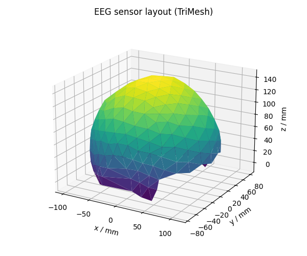
Visualising the EEG sensor mesh

The EEG montage is represented by a triangular surface mesh with vertices at the electrode positions. We plot this mesh once to get a feeling for the spatial sampling layout.

fig = plt.figure(figsize=(6, 5))
ax = fig.add_subplot(111, projection="3d")

# TriMesh exposes vertex and triangle lists; we use them for a trisurf plot.
verts = mesh_eeg.vertlist
tris = mesh_eeg.trilist

# simple colouring: channel index mapped to colormap
colors = np.arange(verts.shape[0])

surf = ax.plot_trisurf(
    verts[:, 0],
    verts[:, 1],
    verts[:, 2],
    triangles=tris,
    cmap="viridis",
    linewidth=0.2,
    antialiased=True,
)

ax.set_title("EEG sensor layout (TriMesh)")
ax.set_xlabel("x / mm")
ax.set_ylabel("y / mm")
ax.set_zlabel("z / mm")
ax.view_init(elev=20, azim=-60)

plt.tight_layout()
plt.show()

Computing a SPHARA basis (FEM discretisation)

The SPHARA basis is obtained by solving a generalised eigenproblem

\[\mathbf{S}\,\boldsymbol{\phi}_i = \tau_i\,\mathbf{B}\,\boldsymbol{\phi}_i,\]

where \(\mathbf{S}\) is a discrete Laplace–Beltrami operator, \(\mathbf{B}\) a symmetric positive definite mass matrix, and \(\tau_i \ge 0\) are the eigenvalues. The eigenvectors \(\boldsymbol{\phi}_i\) form the SPHARA basis functions.

In this example we use the finite element method (FEM) to discretise the Laplace–Beltrami operator. The FEM approach takes into account the geometry of the underlying surface, which is required to obtain spatial frequencies and wavelengths with physical units.

sphara_basis = sb.SpharaBasis(mesh_eeg, mode="fem")
Phi, eigenvalues = sphara_basis.basis()

print(f"Basis matrix shape: {Phi.shape}")
print(f"Number of eigenvalues: {eigenvalues.shape[0]}")

Basis matrix shape: (256, 256)
Number of eigenvalues: 256

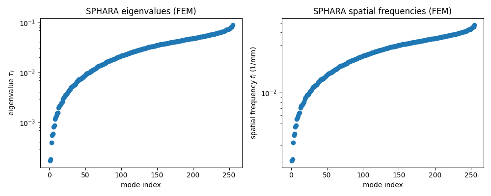
From eigenvalues to spatial frequencies and wavelengths

For a FEM-based Laplace–Beltrami discretisation the eigenvalues \(\tau_i\) are related to spatial wave numbers via

\[\sqrt{\tau_i} = 2\pi f_i = \frac{2\pi}{\lambda_i},\]

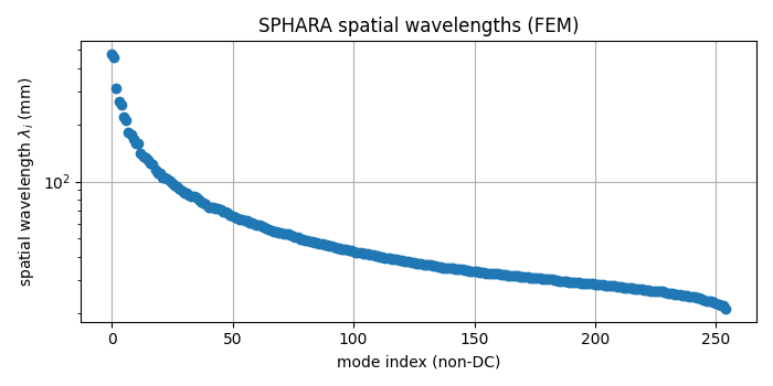
where \(f_i\) denotes the spatial frequency and \(\lambda_i\) the corresponding spatial wavelength. We can therefore derive spatial frequencies and wavelengths directly from the eigenvalues.

tau = np.maximum(eigenvalues, 0.0)  # guard against tiny negative values
spatial_freq = np.sqrt(tau) / (2.0 * np.pi)
spatial_wavelength = np.empty_like(spatial_freq)
non_zero = spatial_freq > 0
spatial_wavelength[non_zero] = 1.0 / spatial_freq[non_zero]
spatial_wavelength[~non_zero] = np.inf  # DC component

Plotting the SPHARA spectrum of the mesh

It can be helpful to inspect the eigenvalues and derived spatial frequencies on a log scale.

fig, axes = plt.subplots(1, 2, figsize=(10, 4))

axes[0].semilogy(tau, marker="o", linestyle="none")
axes[0].set_xlabel("mode index")
axes[0].set_ylabel(r"eigenvalue $\tau_i$")
axes[0].set_title("SPHARA eigenvalues (FEM)")

axes[1].semilogy(spatial_freq, marker="o", linestyle="none")
axes[1].set_xlabel("mode index")
axes[1].set_ylabel(r"spatial frequency $f_i$ (1/mm)")
axes[1].set_title("SPHARA spatial frequencies (FEM)")

plt.tight_layout()
plt.show()

# spatial wavelengths in mm (ignore the infinite DC component)
fig_lambda, ax_lambda = plt.subplots(figsize=(7, 3.5))
ax_lambda.semilogy(spatial_wavelength[non_zero], marker="o", linestyle="none")
ax_lambda.set_xlabel("mode index (non-DC)")
ax_lambda.set_ylabel(r"spatial wavelength $\lambda_i$ (mm)")
ax_lambda.set_title("SPHARA spatial wavelengths (FEM)")
ax_lambda.grid(True)

plt.tight_layout()
plt.show()

• 
• 

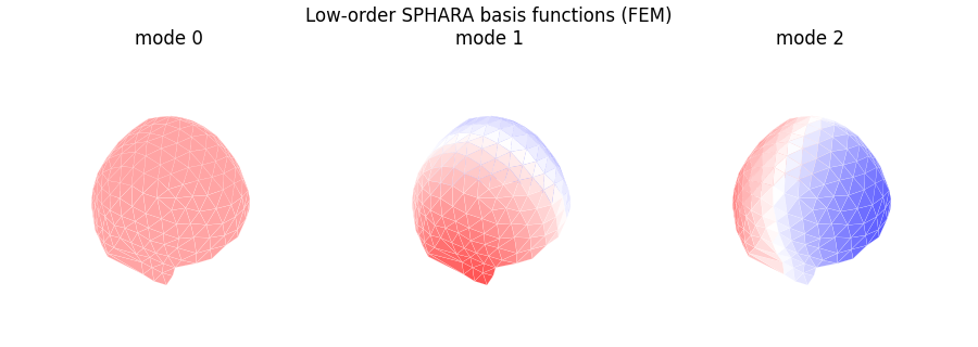
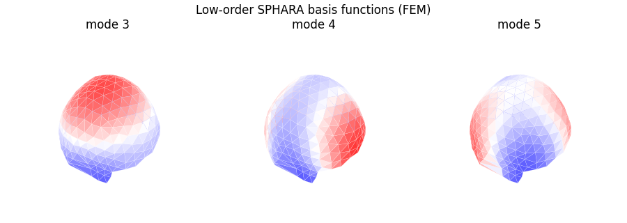
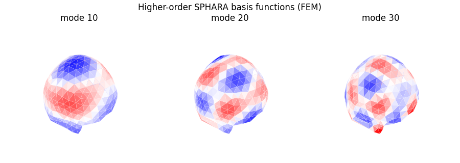
Visualising a few SPHARA basis functions

To build intuition, we now visualise a small number of SPHARA basis functions on the EEG mesh. Low-order basis functions have a smooth spatial variation (large wavelengths), whereas higher-order functions show more oscillations (shorter wavelengths).

def plot_basis_on_mesh(mesh: tm.TriMesh, basis_matrix: np.ndarray, mode_indices, title: str) -> None:
    """Plot selected SPHARA basis functions on a triangulated mesh."""
    verts_loc = mesh.vertlist
    tris_loc = mesh.trilist

    n_modes = len(mode_indices)
    n_rows = 1
    n_cols = n_modes

    fig = plt.figure(figsize=(3.0 * n_cols, 3.2))
    fig.suptitle(title)

    for i, idx in enumerate(mode_indices):
        ax = fig.add_subplot(n_rows, n_cols, i + 1, projection="3d")
        colors = np.mean(basis_matrix[tris_loc, idx], axis=1)
        coeffs = basis_matrix[:, idx]
        surf = ax.plot_trisurf(
            verts_loc[:, 0],
            verts_loc[:, 1],
            verts_loc[:, 2],
            triangles=tris_loc,
            cmap="bwr",
            edgecolor="white",
            linewidth=0.1,
            antialiased=True,
            shade=True,
            vmin=-np.max(np.abs(coeffs)),
            vmax=np.max(np.abs(coeffs)),
        )
        surf.set_array(colors)
        surf.set_clim(-0.01, 0.01)

        ax.set_title(f"mode {idx}")
        ax.set_axis_off()
        ax.view_init(elev=45, azim=-60)

    plt.tight_layout()
    plt.show()


# plot a few low-order basis functions
plot_basis_on_mesh(
    mesh_eeg,
    Phi,
    mode_indices=[0, 1, 2],
    title="Low-order SPHARA basis functions (FEM)",
)

# plot a few low-order basis functions
plot_basis_on_mesh(
    mesh_eeg,
    Phi,
    mode_indices=[3, 4, 5],
    title="Low-order SPHARA basis functions (FEM)",
)

# plot a few higher-order basis functions
plot_basis_on_mesh(
    mesh_eeg,
    Phi,
    mode_indices=[10, 20, 30],
    title="Higher-order SPHARA basis functions (FEM)",
)

• 
• 
• 

SPHARA transform of the EEG data

Once the SPHARA basis has been computed, we can project the EEG data onto this basis. This is achieved via the SPHARA transform class.

The analysis operation maps sensor-space signals \(\boldsymbol{x}(t)\) to SPHARA coefficients \(\boldsymbol{c}(t)\):

\[\boldsymbol{c}(t) = \mathbf{\Phi}^\top \mathbf{B}\,\boldsymbol{x}(t),\]

where \(\mathbf{B}\) is the FEM mass matrix. The inverse operation reconstructs sensor-space data from SPHARA coefficients.

sphara_transform = st.SpharaTransform(mesh_eeg, mode="fem")

# The transform expects samples in rows (n_samples, n_channels).
# Our data are arranged as (n_channels, n_times), so we transpose
# before and after the transform.

eeg_data_T = eeg_data.T  # shape (n_times, n_channels)
coeffs = sphara_transform.analysis(eeg_data_T)        # (n_times, n_channels)
eeg_recon_T = sphara_transform.synthesis(coeffs)      # (n_times, n_channels)
eeg_recon = eeg_recon_T.T                             # back to (n_channels, n_times)

Reconstruction check

For an orthonormal SPHARA basis and full-rank transform, analysis followed by synthesis should reconstruct the original data up to numerical precision. We verify this by computing the maximum absolute reconstruction error.

max_abs_error = np.max(np.abs(eeg_data - eeg_recon))
print(f"Maximum absolute reconstruction error: {max_abs_error:.3e}")

Maximum absolute reconstruction error: 1.066e-14

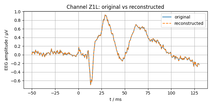
Visual comparison at a single channel

To see the reconstruction quality in the time domain, we select a single channel and overlay the original and reconstructed signals.

channel_index = 0  # first channel

# time axis in milliseconds: 50 ms before to 130 ms after stimulation
t_ms = np.linspace(-50.0, 130.0, n_times)

fig, ax = plt.subplots(figsize=(7, 3.5))
ax.plot(t_ms, eeg_data[channel_index, :], label="original")
ax.plot(t_ms, eeg_recon[channel_index, :], linestyle="--", label="reconstructed")
ax.set_xlabel("t / ms")
ax.set_ylabel("EEG amplitude / µV")
ax.set_title(f"Channel {channel_labels[channel_index]}: original vs reconstructed")
ax.grid(True)
ax.legend()

plt.tight_layout()
plt.show()

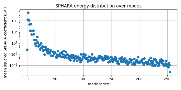
SPHARA coefficient energy over mode index

Finally, we examine how the energy of the EEG data is distributed over the SPHARA modes. For each mode \(i\) we compute the mean squared coefficient magnitude across time and plot it as a function of the mode index.

coeffs_T = coeffs.T  # shape (n_channels, n_times)
mode_energy = np.mean(np.abs(coeffs_T) ** 2, axis=1)

fig, ax = plt.subplots(figsize=(7, 3.5))
ax.semilogy(mode_energy, marker="o", linestyle="none")
ax.set_xlabel("mode index")
ax.set_ylabel("mean squared SPHARA coefficient (µV²)")
ax.set_title("SPHARA energy distribution over modes")
ax.grid(True)

plt.tight_layout()
plt.show()

Summary and outlook

In this tutorial we have

• constructed a SPHARA basis for a triangulated EEG layout using a FEM discretisation of the Laplace–Beltrami operator,

• derived spatial frequencies and wavelengths from the eigenvalues,

• visualised low- and high-order SPHARA basis functions, and

• computed and verified the SPHARA transform of multichannel EEG data.

In the next tutorial we will design SPHARA-domain filters (ideal, Gaussian, Butterworth) using the spharapy.spectral_filters module and apply them to EEG data, including noise-robust spatial low-pass filtering.