SPHARA spatial filtering of EEG data (BaCI 2019)

Based on the course materials from Training Course 4, held at the International Conference on Basic and Clinical Multimodal Imaging (BaCI) in Chengdu, China, in September 2019.

In the previous tutorial we computed a SPHARA basis for a 256-channel EEG montage using a finite-element (FEM) discretisation of the Laplace–Beltrami operator, derived spatial frequencies and wavelengths from the eigenvalues, and applied the SPHARA transform to multichannel somatosensory evoked potential (SEP) data.

In this tutorial we use that SPHARA representation to design and apply spatial filters in the SPHARA domain:

• ideal (brick-wall) low-pass filters,

• Gaussian low-pass filters, and

• Butterworth low-pass filters.

We will compare their transfer functions, apply them to the SEP data, and demonstrate spatial smoothing in the presence of additive sensor noise.

The example data set contains 256-channel SEP recordings with vertex positions given in millimetres (mm) and EEG amplitudes measured in microvolts (µV). The recording consists of 369 samples from 50 ms before to 130 ms after stimulation at a sampling frequency of 2048 Hz.

Imports and dataset

import numpy as np
import matplotlib.pyplot as plt
from mpl_toolkits.mplot3d import Axes3D  # noqa: F401  (required for 3D plotting)

import spharapy.datasets as sd
import spharapy.trimesh as tm
import spharapy.spharabasis as sb
import spharapy.spharafilter as sf
from spharapy.spectral_filters import (
    transfer_func_ideal_lowpass,
    transfer_func_gaussian_lowpass,
    transfer_func_butterworth_lowpass,
)

We use the same 256-channel SEP data set as in examples.plot_04_sphara_filter_eeg. The loader returns a dictionary with vertex list, triangle list, EEG data and channel labels.

mesh_in = sd.load_eeg_256_channel_study()

print(mesh_in.keys())

vertlist = np.array(mesh_in["vertlist"])
trilist = np.array(mesh_in["trilist"])
labelist = np.array(mesh_in["labellist"])
eegdata = np.array(mesh_in["eegdata"])

# channel labels
channel_labels = labelist

print("vertices = ", vertlist.shape)
print("triangles = ", trilist.shape)
print("eegdata = ", eegdata.shape)

# build TriMesh and standardised variable names used in this tutorial
mesh_eeg = tm.TriMesh(trilist, vertlist)
eeg_data = eegdata  # shape (n_channels, n_times)

n_channels, n_times = eeg_data.shape

dict_keys(['vertlist', 'trilist', 'labellist', 'eegdata'])
vertices =  (256, 3)
triangles =  (482, 3)
eegdata =  (256, 369)

Construct SPHARA basis and spatial frequency axis

As in the first tutorial, we construct a SPHARA basis using the FEM discretisation of the Laplace–Beltrami operator. The eigenvalues \(\tau_i \ge 0\) are converted into spatial frequencies \(f_i\) (in 1/mm) via

\[\sqrt{\tau_i} = 2\pi f_i.\]

These spatial frequencies provide a natural axis for designing SPHARA-domain filters.

sphara_basis = sb.SpharaBasis(mesh_eeg, mode="fem")
Phi, eigenvalues = sphara_basis.basis()

tau = np.maximum(eigenvalues, 0.0)
spatial_freq = np.sqrt(tau) / (2.0 * np.pi)  # in 1/mm

f_min = float(np.min(spatial_freq))
f_max = float(np.max(spatial_freq))

print(f"Spatial frequency range: [{f_min:.3e}, {f_max:.3e}] 1/mm")

Spatial frequency range: [0.000e+00, 4.745e-02] 1/mm

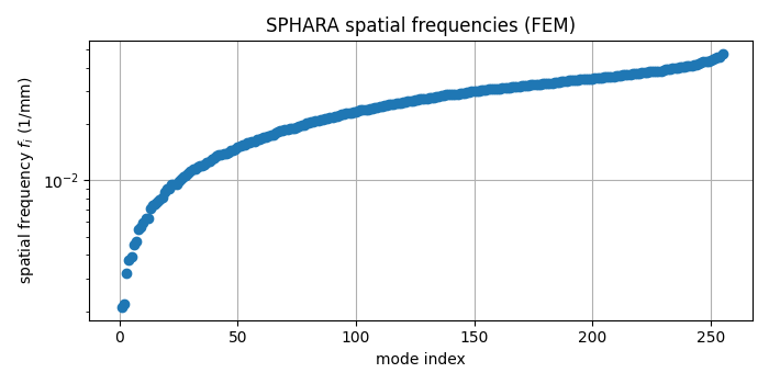
Visualising the spatial frequency grid

Each SPHARA mode is associated with a spatial frequency. We visualise this grid, which will form the x-axis for the transfer functions of our filters.

fig, ax = plt.subplots(figsize=(7, 3.5))
ax.semilogy(spatial_freq, marker="o", linestyle="none")
ax.set_xlabel("mode index")
ax.set_ylabel(r"spatial frequency $f_i$ (1/mm)")
ax.set_title("SPHARA spatial frequencies (FEM)")
ax.grid(True)

plt.tight_layout()
plt.show()

Designing SPHARA low-pass filters

We now design three different low-pass filters in the SPHARA domain:

• an ideal (brick-wall) low-pass filter,

• a Gaussian low-pass filter, and

• a Butterworth low-pass filter.

All transfer functions are expressed as functions of the spatial frequency \(f_i\). For illustration we choose a cut-off at \(f_c = 0.2 \, f_\mathrm{max}\).

f_rel_cut = 0.2  # relative cutoff
fc = f_rel_cut * f_max

print(f"Using low-pass cutoff fc = {fc:.3e} 1/mm  (~{f_rel_cut:.0%} of max f)")

# Ideal low-pass
H_ideal = transfer_func_ideal_lowpass(spatial_freq, fc=fc)

# Gaussian low-pass: half-power at fc
H_gauss = transfer_func_gaussian_lowpass(
    spatial_freq,
    fc=fc,
    dB=-3.01029995664,  # ≈ half-power
)

# Butterworth low-pass of moderate order
H_butt = transfer_func_butterworth_lowpass(
    spatial_freq,
    fc=fc,
    order=4,
    dB=-3.01029995664,
)

Using low-pass cutoff fc = 9.489e-03 1/mm  (~20% of max f)

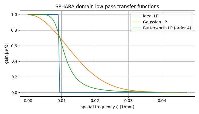
Comparing transfer functions

We plot the three transfer functions versus the spatial frequency axis. This highlights the differences between sharp (ideal), smoothly decaying (Gaussian), and more gradually transitioning (Butterworth) responses.

fig, ax = plt.subplots(figsize=(7, 4))

ax.plot(spatial_freq, H_ideal, label="ideal LP")
ax.plot(spatial_freq, H_gauss, label="Gaussian LP")
ax.plot(spatial_freq, H_butt, label="Butterworth LP (order 4)")

ax.set_xlabel(r"spatial frequency $f_i$ (1/mm)")
ax.set_ylabel(r"gain $|H(f_i)|$")
ax.set_title("SPHARA-domain low-pass transfer functions")
ax.grid(True)
ax.legend()

plt.tight_layout()
plt.show()

Building SPHARA filters and applying them to SEP data

The transfer functions \(H(f_i)\) can be used as filter specifications (one gain value per SPHARA mode) in spharapy.spharafilter.SpharaFilter. Internally the class will

• construct a SPHARA basis for the mesh (if not yet available),

• transform the data into the SPHARA domain,

• apply the spectral gains, and

• transform the data back to sensor space.

The filter() method expects data with samples in rows and channels in columns. Our data are stored as (n_channels, n_times), so we transpose before filtering.

# Helper to apply a SPHARA filter and return (n_channels, n_times)
def apply_sphara_filter(mesh: tm.TriMesh, specification: np.ndarray, data: np.ndarray) -> np.ndarray:
    filt = sf.SpharaFilter(mesh, mode="fem", specification=specification)
    data_T = data.T  # (n_times, n_channels)
    data_filt_T = filt.filter(data_T)
    return data_filt_T.T  # back to (n_channels, n_times)


eeg_ideal = apply_sphara_filter(mesh_eeg, H_ideal, eeg_data)
eeg_gauss = apply_sphara_filter(mesh_eeg, H_gauss, eeg_data)
eeg_butt = apply_sphara_filter(mesh_eeg, H_butt, eeg_data)

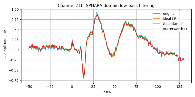
Visual comparison at a single channel

We select one example channel and compare the original SEP waveform to the three filtered versions. The time axis is expressed in milliseconds.

channel_index = 0  # first channel

t_ms = np.linspace(-50.0, 130.0, n_times)

fig, ax = plt.subplots(figsize=(8, 4))
ax.plot(t_ms, eeg_data[channel_index, :], label="original", alpha=0.7)
ax.plot(t_ms, eeg_ideal[channel_index, :], label="ideal LP")
ax.plot(t_ms, eeg_gauss[channel_index, :], label="Gaussian LP")
ax.plot(t_ms, eeg_butt[channel_index, :], label="Butterworth LP")

ax.set_xlabel("t / ms")
ax.set_ylabel("EEG amplitude / µV")
ax.set_title(f"Channel {channel_labels[channel_index]}: SPHARA-domain low-pass filtering")
ax.grid(True)
ax.legend(loc="best")

plt.tight_layout()
plt.show()

Energy distribution before and after filtering

To quantify the effect of the filters in the SPHARA domain, we compute the mean squared amplitude of each channel over time and sum this across channels. This yields a global measure of signal energy in sensor space, expressed in µV².

def total_energy(data: np.ndarray) -> float:
    """Return total energy (sum of squared amplitudes) in µV²."""
    return float(np.sum(np.abs(data) ** 2))


E_orig = total_energy(eeg_data)
E_ideal = total_energy(eeg_ideal)
E_gauss = total_energy(eeg_gauss)
E_butt = total_energy(eeg_butt)

print(f"Total energy original:   {E_orig:.3e} µV²")
print(f"Total energy ideal LP:   {E_ideal:.3e} µV²")
print(f"Total energy Gaussian:   {E_gauss:.3e} µV²")
print(f"Total energy Butterworth:{E_butt:.3e} µV²")

Total energy original:   1.250e+04 µV²
Total energy ideal LP:   1.213e+04 µV²
Total energy Gaussian:   1.052e+04 µV²
Total energy Butterworth:1.203e+04 µV²

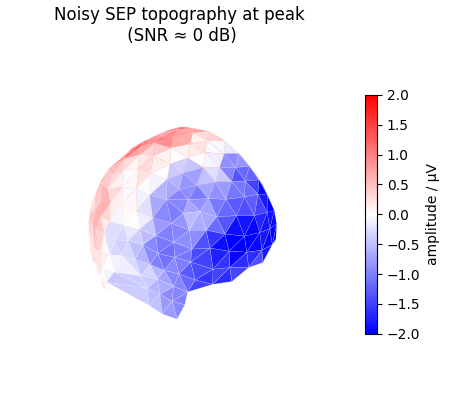
Adding noise and demonstrating spatial smoothing

To illustrate the spatial smoothing effect of SPHARA low-pass filtering, we now add synthetic sensor noise to the SEP data and compare topographic maps at the SEP peak.

We generate zero-mean Gaussian noise such that the resulting global signal-to-noise ratio (SNR) is approximately 0 dB, i.e. signal and noise have comparable power.

rng = np.random.default_rng(seed=42)

# target SNR in dB
snr_db = 0.0
snr_lin = 10.0 ** (snr_db / 10.0)

# noise variance chosen such that signal_power / noise_power ≈ snr_lin
signal_power = np.mean(eeg_data**2)
noise_power = signal_power / snr_lin
noise_std = np.sqrt(noise_power)

noise = rng.normal(loc=0.0, scale=noise_std, size=eeg_data.shape)
eeg_noisy = eeg_data + noise

print(f"Approximate signal power: {signal_power:.3e} µV²")
print(f"Approximate noise power:  {noise_power:.3e} µV²")

# filter the noisy data with the Gaussian low-pass filter
eeg_noisy_gauss = apply_sphara_filter(mesh_eeg, H_gauss, eeg_noisy)

Approximate signal power: 1.323e-01 µV²
Approximate noise power:  1.323e-01 µV²

Helper: plot scalar field on the EEG mesh

def plot_scalar_on_mesh(mesh: tm.TriMesh, values: np.ndarray, title: str) -> None:
    """Plot a scalar quantity defined at mesh vertices on a 3D triangulated surface."""
    verts_loc = mesh.vertlist
    tris_loc = mesh.trilist

    fig = plt.figure(figsize=(4.5, 4))
    ax = fig.add_subplot(111, projection="3d")

    #val = np.asarray(values, dtype=float)
    val = np.mean(values[tris_loc], axis=1)
    vmax = np.max(np.abs(val)) or 1.0

    surf = ax.plot_trisurf(
        verts_loc[:, 0],
        verts_loc[:, 1],
        verts_loc[:, 2],
        triangles=tris_loc,
        cmap="bwr",
        edgecolor="white",
        linewidth=0.1,
        antialiased=True,
        shade=True,
        vmin=-vmax,
        vmax=vmax
    )

    surf.set_array(val)
    surf.set_clim(-2.0, 2.0)

    ax.set_title(title)
    ax.set_axis_off()
    ax.view_init(elev=30, azim=-60)

    fig.colorbar(surf, ax=ax, shrink=0.7, label="amplitude / µV")

    plt.tight_layout()
    plt.show()

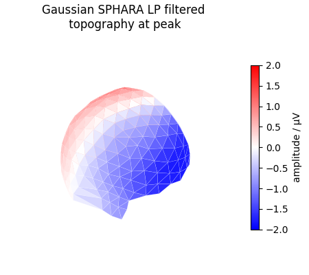
Topographic maps at the SEP peak

We determine the global peak over time (maximising the ℓ2-norm across channels) and plot topographic maps for:

• the original SEP data,

• the noisy data, and

• the Gaussian low-pass filtered noisy data.

# index of time sample with maximal global amplitude
peak_index = int(np.argmax(np.linalg.norm(eeg_data, axis=0)))

print(f"Peak sample index: {peak_index}  (~t = {t_ms[peak_index]:.1f} ms)")

topo_orig = eeg_data[:, peak_index]
topo_noisy = eeg_noisy[:, peak_index]
topo_filt = eeg_noisy_gauss[:, peak_index]

plot_scalar_on_mesh(mesh_eeg, topo_orig, "Original SEP topography at peak")
plot_scalar_on_mesh(mesh_eeg, topo_noisy, "Noisy SEP topography at peak\n (SNR ≈ 0 dB)")
plot_scalar_on_mesh(mesh_eeg, topo_filt, "Gaussian SPHARA LP filtered\n topography at peak")

• 
• 
• 

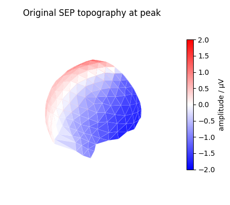
Peak sample index: 163  (~t = 29.7 ms)

Summary

In this tutorial we have demonstrated how to design and apply spatial filters in the SPHARA domain using SpharaPy:

• SPHARA eigenvalues (for a FEM Laplace–Beltrami discretisation) were converted into spatial frequencies \(f_i\) in 1/mm.

• Ideal, Gaussian, and Butterworth low-pass transfer functions were defined as functions of \(f_i\) using spharapy.spectral_filters.

• These transfer vectors were used as specifications for spharapy.spharafilter.SpharaFilter to perform SPHARA-domain filtering.

• We compared the temporal response at a single EEG channel and the spatial energy in µV² before and after filtering.

• In a noisy setting (SNR ≈ 0 dB), Gaussian SPHARA low-pass filtering produced visibly smoother and more interpretable topographic maps at the SEP peak.

More advanced designs (e.g., high-pass or band-pass filters, or filters tuned to specific spatial frequency bands) can be obtained by combining the low-pass transfer functions or using the helper functions provided in spharapy.spectral_filters.